ADAP-BIG v1.6.0 User Manual
Introduction
ADAP Informatics Ecosystem
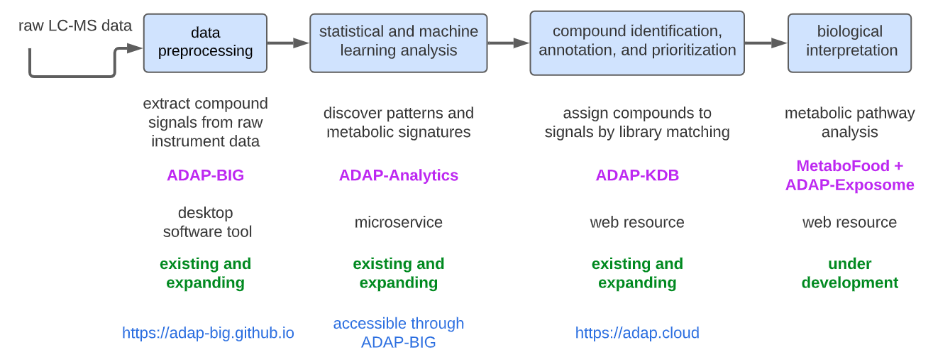
ADAP-BIG is a part of the ADAP informatics ecosystem, a collection of software tools for processing and analyzing mass spectrometry data. The ADAP informatics ecosystem consists of the following software tools (Figure 1.1):
ADAP-BIG is a software tool for processing raw gas chromatography (GC-) and liquid chromatography coupled to mass spectrometry (LC-MS) data. It can produce a CSV file with the detected features, their retention times and intensities, and an MSP file with spectra of the detected features.
ADAP-Analytics is a software tool for analyzing the processed data from ADAP-BIG. It can perform statistical tests, such as ANOVA, PCA, and PLS-DA. Currently, ADAP-Analytics is accessible through ADAP-BIG only (see Chapter 6).
ADAP-KDB is a web application for compound identification, annotations, and prioritization. The spectra of the detected features from ADAP-BIG can be uploaded to ADAP-KDB (https://adap.cloud) to perform library matching against publicly available and user-provided private spectral libraries.
MetaboFood + ADAP-Exposome is a web resource for biological interpretation of metabolomics data. This resource is currently under development and will be available in the future.
The ADAP informatics ecosystem is designed to provide a comprehensive solution for processing, analyzing, and interpreting mass spectrometry data. The ecosystem is developed by the Du-lab team at the University of North Carolina at Charlotte in collaboration with other research groups from University of North Carolina at Chapel Hill and University of Arkansas for Medical Sciences. For more information about the ADAP informatics ecosystem, please visit the Du-lab website at http://www.dulab.org.
ADAP-BIG is free software designed to handle a large number of samples on machines with minimal system requirements. It features a user-friendly graphical interface that provides visualization of raw data and intermediate results for each step of the data processing. The software is cross-platform and can be used on Windows, Mac OS, and Linux. Although ADAP-BIG is a part of the ADAP informatics ecosystem, it can be used as a standalone software tool for processing raw untargeted mass spectrometry data. Users can import raw data files, process them using one of the available workflows, and export the processing results to CSV and MSP files for further analysis. The exported feature tables and spectra can be imported into ADAP-KDB or other third-party software tools for compound identification and/or statistical analysis.
Download and Installation
ADAP-BIG is a cross-platform desktop application, that can be used on Windows, Mac OS, and Linux. Users can download a platform-specific installation package to easily install the application on their workstations. To download the installation package for your platform, please visit the GitHub Release page. Table 1.1 provides the list of files available for download.
| File | Description |
|---|---|
| Adap-Big App-x.x.x.exe | Installation package that installs ADAP-BIG application on Windows. |
| Adap-Big App-x.x.x.pkg | Installation package that installs ADAP-BIG application on Mac OS. |
| adap-big-app_x.x.x-1_amd64.deb | Installation package that installs ADAP-BIG application on Linux (Ubuntu). |
| adap-big-app_x.x.x-1_amd64.rpm | Installation package that installs ADAP-BIG application on Linux (CentOS). |
| adap-big-console-app-x.x.x.jar | Console application to run ADAP-BIG in a terminal (Require Java 9+). |
| adap-big-jar-files-x.x.x.zip | Collection of individual jar files for each workflow step (Require Java 9+). |
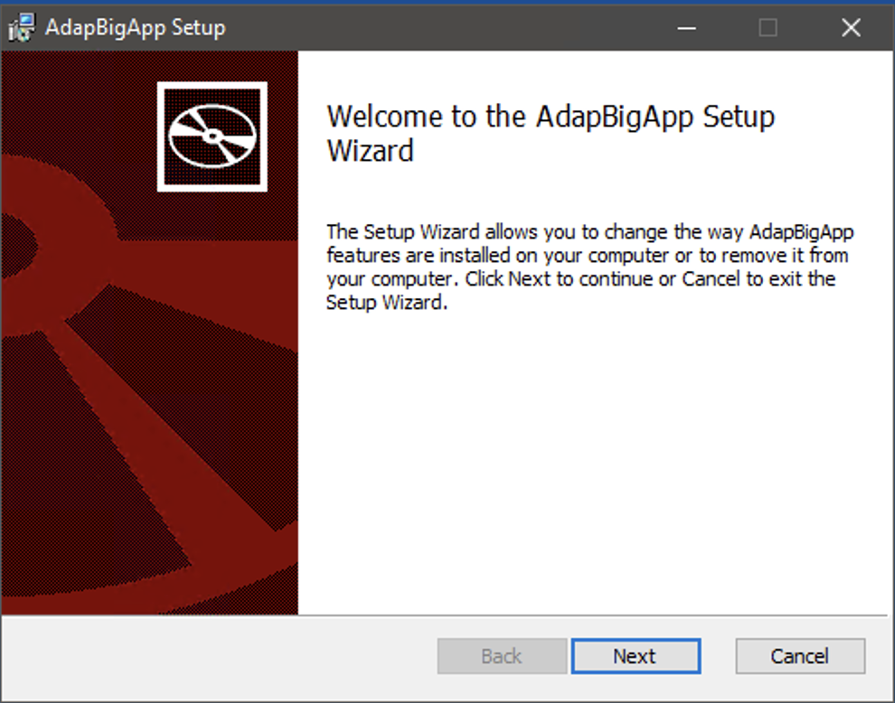
Installation of ADAP-BIG on Windows.
Download file Adap-Big App-x.x.x.exe from the GitHub Release page.
Start the installation process by double-clicking on the downloaded file.
If you get the message that Microsoft Defender prevented an unrecognized app from starting, please click “More info” and “Run anyway”to continue. If you do not see the “More info” button, please contact your system administrator to allow the installation of the application.
Run ADAP-BIG by clicking the Windows Start Button and selecting the ADAP-BIG application.
Installation of ADAP-BIG on Mac OS
Download file Adap-Big App-x.x.x.pkg from the GitHub Release page.
Start the installation process by double-clicking on the downloaded file.
If you get the message that the application cannot be opened because it is from an unidentified developer, go to System Settings/Privacy and Security, find the line with Adap-Big App-x.x.x.pkg, and click "Open Anyway." If this option is not available, please contact your system administrator to allow the installation of the application.
Run ADAP-BIG from the Launchpad or the Applications folder in Finder.
Installation of ADAP-BIG on Linux
Download file adap-big-app_x.x.x_amd64.deb (if the Linux system is Debian-based) or file adap-big-app-x.x.x-1.x86_64.rpm (if the Linux system is Red-Hat-based) from the GitHub Release page.
Start the installation process by double-clicking on the downloaded file. The installation process depends on what Linux system is used, but usually the double-clicking on the downloaded file will open the system package manager, where you will be able to click the “Install” button.
Run ADAP-BIG from the start menu or the applications folder (depending on what Linux system is used).
User Interface
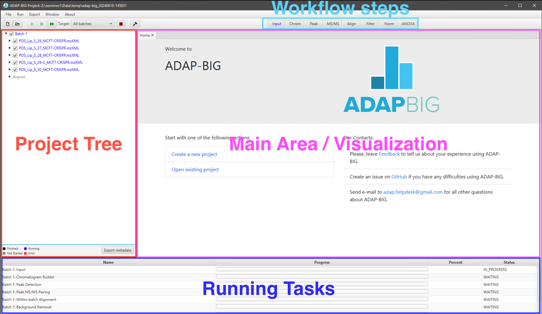
User interface of ADAP-BIG is shown on Figure 1.2 and consists of the main area, project tree (left-hand side of the application window), workflow bar (top of the application window), and progress area (bottom of the application window). When the application is just started, the project tree, workflow bar, and progress area will be empty since no project is currently open in ADAP-BIG, and the main area will show a home page with a contact information and buttons to create a new project or open an existing project.
After a project is created or opened in ADAP-BIG, the project tree displays batch names (Batch 1, Batch 2, Batch 3,…), sample names (based on the raw data filenames), and workflow steps (Input, Chromatogram Builder, Peak Detection,…) of that project. Users may need to expand batch and sample items to see their workflow steps in the project tree. Alternatively, users can see all workflow steps in the workflow bar at the top of the application window. All items in the project tree and the workflow bar are color-coded: black means that the processing of a specific workflow step on a specific sample is completed, blue means that the processing is currently running, gray means that the processing has not started yet, and red means that the processing resulted in an error. In addition to the color-coded items in the project tree and workflow bar, users can see the currently running workflow step and all queued steps in the progress area at the bottom of the application window.
To view the raw data or processing results of a workflow step, users can select a workflow step by clicking one of the items either in the workflow bar or in the project tree. This will open a new tab with the visualization of that workflow step in the main area. See later sections of the manual for more details on visualization of each workflow step. In order to see the final processing results, users just need to select the last step in a workflow. While the project tree and workflow bar are similar in their functionality, the project tree is more detailed and let users view the processing results of a particular step on a particular sample, while the workflow bar let users select only a workflow step but not a sample. However, the workflow bar is much easier to navigate.
When a workflow step is performed on each sample individually (e.g., Chromatogram Builder or Peak Detector), the processing results will be shown only for a single sample. Users can see the name of that sample in the tab header, and that sample will be highlighted in the project tree. Users are advised to wait until a workflow step has finished before viewing its processing results. Otherwise, they will see a message saying that the processing results are not available yet and asking to rerun that workflow step.
Performance and System Requirements
ADAP-BIG is a Java-based desktop application that can be run on Windows, Mac OS, and Linux. In addition, ADAP-BIG can be run in a terminal and on a high-performance cluster via the console application (see Section 2.6). The system requirements for running ADAP-BIG depend on the size of the raw data files, and the number of samples in the project, the workflow used for processing the data, and individual parameters of the workflow steps.
In order to demonstrate the system requirements for processing raw mass spectrometry data with ADAP-BIG, we evaluated the performance of ADAP-BIG with three different datasets:
1 batch, 88 samples with 8.8 GB of raw data files;
15 batches, 1,389 samples with 132 GB of raw data files;
51 batches, 5,271 samples with 503 GB of raw data files.
| Number of produced features | ||||
| 1 sample | 1 batch | 15 batches | 51 batches | |
| Single-batch steps | ||||
| Chromatogram Builder | 15,555 | |||
| Peak Detection | 84,309 | |||
| MS/MS Pairing | 84,309 | |||
| Join Aligner | 430,553 | |||
| Background Removal | 36,717 | |||
| Multi-batch steps | ||||
| Between Batch Aligner | 13,821 | 12,542 | ||
| Normalization | 13,821 | 12,542 | ||
| Batch Effect Correction | 13,821 | 12,542 | ||
| Multi-Batch Pool RSD Filter | ||||
For processing these three datasets, we used the single batch LC-MS/MS workflow for Dataset 1 and the multi-batch LC-MS/MS workflow for Datasets 2 and 3 with the default parameters (see Sections 3.2, 3.3 for more details). The processing steps in these workflows are listed in Table 1.2 together with the number of produced features after each step of the workflow. We will discuss how the workflow and the number of produced features affect the processing time and system requirements later in this section.
| CPU | RAM | Storage | Year | |
|---|---|---|---|---|
| Laptop | Apple M3 | 16 GB | 1 TB | 2024 |
| 8 cores | LPDDR5 | SSD | ||
| max. 4.05 GHz | 3200 MHz | max. 7.4 GB/s | ||
| Workstation | Intel Xeon W-2145 | 64 GB | 800 GB | 2018 |
| 8 cores | DDR4 | SSD | ||
| max. 4.50 GHz | 2666 MHz | PCIe 3 | ||
| Server | AMD EPYC 7313P | 512 GB | 1 TB | 2023 |
| 16 cores | DDR4 | NVMe | ||
| max. 3.70 GHz | 3200 MHz | PCIe 4 |
Finally, the machines used for testing ADAP-BIG are listed in Table 1.3. The first machine is a MacBook with an Apple M3 processor, while the second and third machines are high-performance workstation with Intel Xeon W-2145 and server with AMD EPYC 7313P processor, respectively. The Macbook is the newest generation of Apple laptops (at the moment of writing), while the workstation and server are several years old. Because of these machines are several years apart, the performance between them is not directly comparable. Therefore, readers are encouraged to use the performance results as examples of the processing times and system requirements for different datasets, rather than as a direct comparison of the performance between Apple and Windows, or between laptops, workstations and servers.
| Laptop | Workstation | Server | |
|---|---|---|---|
| Dataset 1 | 39 min | 46 min | 33 min |
| Dataset 2 | 13 hours | 12 hours | 10 hours |
| Dataset 3 | 2 days, 1 hour | 1 day, 21 hour | 1 day, 11 hours |
The times for ADAP-BIG to process the datasets on different machines are shown in Table 1.4. The processing time is measured from the moment when the user clicks the “Create” button to create a new project until the moment when the last workflow step is completed. The processing time does not include the time for downloading and installing ADAP-BIG, and converting raw data files into the supported formats.
The table shows that the processing time increases with the number of samples and the size of the raw data files. For example, a project with 88 samples and 8.8 GB of raw data files takes about 39 minutes to process on the laptop with an Apple M3 processor and 16 GB of RAM. In contrast, a project with 5,271 samples and 503 GB of raw data files takes about 2 days and 1 hour to process on the same machine. The processing time is reduced on machines with more RAM and cores. For example, the server with AMD EPYC 7313P processor and 512 GB of RAM is able to process 51 batches in about 14 hours faster than the laptop, while the workstation with Intel Xeon W-2145 processor and 64 GB of RAM was only 4 hours faster when processing 51 batches.
There are multiple factors that affect the performance of ADAP-BIG:
CPU and number of cores: The performance of ADAP-BIG is highly dependent on the CPU and the number of cores. The more cores the CPU has, the faster the processing will be. For example, the server with AMD EPYC 7313P processor has 16 cores and is able to process 51 batches in about 1 day and 11 hours, while the workstation with Intel Xeon W-2145 processor has only 8 cores and takes about 1 day and 21 hours to process the same dataset.
Available RAM: The machine has to have enough RAM for processing with ADAP-BIG, otherwise the processing will freeze or completely fail. We recommend having at least 4 GB per core. It is remarkable that even the laptop with 2 GB per core was able to process all 51 batches of the data in our tests. However, whether 2 GB per core is enough or not depends on the size of the raw data files, processing workflow and parameters. For example in our tests, the Background Removal step reduced the number of features by 90% (see Table 1.2), which significantly improved performance of ADAP-BIG. If the Background Removal step is not used (or the dataset doesn’t contain blank and pool samples required by the Background Removal), the performance of ADAP-BIG will be worse.
Fast Storage: The ADAP-BIG performs frequent writing data to and reading data from disk. Therefore, the performance of ADAP-BIG is also dependent on the speed of the storage. In our tests, the laptop had the fastest storage, and as a result, it was able to show similar performance to the workstation and the server with slower storage, especially when processing the Dataset 1 with only 88 samples.
In summary, ADAP-BIG can be run on a laptop with 16 GB of RAM and 4 cores, but for processing large datasets with thousands of samples, we recommend using a workstation or server with at least 64 GB of RAM and 8 cores. The performance of ADAP-BIG is highly dependent on the CPU, number of cores, available RAM, and speed of the storage. It is important to note that the performance of ADAP-BIG also depends on the size of the raw data files, the number of samples in the project, the workflow used for processing the data, and individual parameters of the workflow steps. Therefore, the performance results presented in this section should only be used as examples of expected performance of ADAP-BIG with a certain workflow and dataset.
Providing Feedback and Reporting Errors
If users want to provide feedback and/or suggestions about ADAP-BIG, they are encouraged to take a short survey by going to https://forms.gle/DqhxF3sfxghv7jNk8. This survey will help the ADAP-BIG team to improve the software and make it more user-friendly. Users can provide feedback on any aspect of ADAP-BIG, including the user interface, data processing, visualization, and documentation. Users can also email their feedback and suggestions to adap.helpdesk@gmail.com.
If users encounter any issues while using ADAP-BIG, they can check the log files for error messages. The log files can be found in two locations:
ADAP-BIG project directory (selected during the
project creation): the log file for the current project is located in
the project directory and has the name adap-big.log. This
log file will contain the log messages for the current project,
including error messages and warnings, from the moment that project was
created. If a project was opened and processed multiple times, the log
file will contain messages from all processing runs.
User home directory: depending on the operating
system, the log files may be located in
C:\Users\USERNAME\.adap-big\logs on Windows, or they can be
located in /home/USERNAME/.adap-big/logs on Linux and
macOS. These log files will contain all messages, warnings, and errors
from all projects created or opened on the computer. Because the number
of messages can become quite large, these log files are split into
groups based on the year and month of the log messages. For example, the
log file for October 2023 will be stored in folder 2023-10.
This helps in managing and reviewing the logs more efficiently. The
current-date messages are still contained in the
adap-big.log file.
Users can open any log file in a text editor to view the error messages and try to identify the cause of the issue. If users are unable to resolve the issue on their own, they can report the error to the ADAP-BIG team by sending an email to adap.helpdesk@gmail.com. In the email, users should describe the issue they encountered, provide the log file with the error messages, and include any other relevant information that may help in diagnosing the problem. The ADAP-BIG team will review the error report and provide assistance in resolving the issue.
Alternatively, users can report the issue by going to https://github.com/ADAP-BIG/adap-big.github.io/issues and clicking the New Issue button. Users have to have a GitHub account in order to create a new issue. In the issue description, users should provide the same information as in the email: a description of the issue, the log file with the error messages, and any other relevant information. The ADAP-BIG team will review the issue and provide assistance in resolving the problem.
Processing Raw MS Data with ADAP-BIG
Supported Raw Data
ADAP-BIG accepts raw data files in the following formats: CDF, mzML, mzXML, and ThermoFisher RAW. The CDF, mzML, and mzXML formats are open formats that can be easily opened and read by many software packages including ADAP-BIG. The ThermoFisher RAW format is a proprietary format used by ThermoFisher mass spectrometers. When ADAP-BIG imports ThermoFisher RAW files, it will internally convert them into the mzML format and then read those mzML files. This conversion is natively supported on Windows systems, but on Mac OS and Linux systems, users need to additionally install the Mono library (https://www.mono-project.com/) if they want to be able to read ThermoFisher RAW files on Mac OS or Linus.
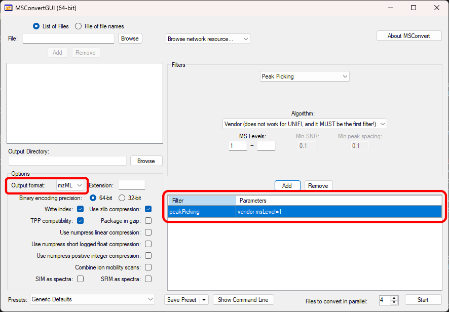
If users have raw data files in other formats, they should use third-party software to convert the data into one of the supported formats. For example, the ProteoWizard package contains a tool called MSConvert that can read from and write to many open and proprietary data formats (Figure 2.1). We highly recommend using MSConvert to convert raw LC-MS data into the mzML format before importing it into ADAP-BIG. For more information about the ProteoWizard package, please visit the ProteoWizard website. Unfortunately, MSConvert does not support converting raw GC-MS data into CDF format, so users need to consult the documentation of their instrument-specific software to find out how to export its raw GC-MS data files into the CDF format.
Finally, ADAP-BIG requires the raw data files to be in the centroid mode. Users can tell whether their raw data is in the profile or centroid mode by viewing it in a mass spectrometry data viewer, e.g. SeeMS from the ProteoWizard package. When zooming in on a single m/z peak, users will see a bell-like shape of the peak if the data is in the profile mode (Figure 2.2, left), or a single horizontal line if the data is in the centroid mode (Figure 2.2, right).
If the raw data is in the profile mode, users can use MSConvert to centroid the data by adding “Peak Picking” to the list of filters when converting their raw data. The Figure 2.1 shows the setup to convert the data into the centroid mode and save it in the mzML format. If the raw data is in the ThermoFisher RAW format, ADAP-BIG will centroid the data automatically. If the raw data is in the CDF format, it is already in the centroid mode and can be imported directly into ADAP-BIG. For more information about MSConvert and its functions, please visit the ProteoWizard website.
Creating a New Project
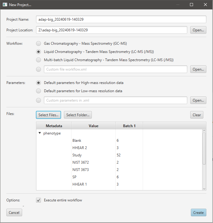
Processing raw data starts with creating a new ADAP-BIG project. Users have multiple options to start a new project: clicking Create a new project button on the home page, selecting New Project... in the main menu, or clicking the corresponding button in the toolbar. After any of these actions, a new window will pop up (Figure 2.3).
First, users are asked to choose name and location of the new project. The name of the project is automatically generated to contain the current date and time, but users may change that name to anything that works for them. The location of the project is automatically set to the user’s home directory (if it is the first launch of ADAP-BIG) or to the previously used location, but can also be updated by a user. Next, users can choose between GC-MS, single-batch LC-MS/MS, multi-batch LC-MS/MS, and custom workflows. If a custom workflow is used, users must choose the XML file that contains the workflow description. See Chapter 3 for more information about each workflow and how to create a custom workflow.
| GC-MS | LC-MS/MS | Multi-batch LC-MS/MS |
|---|---|---|
|
|
|
Table 2.1 shows the three available workflows for processing raw untargeted mass spectrometry data and descriptions of the main workflow steps. The GC-MS workflow consists of the input step, extracted-ion chromatogram (EIC) builder, peak detection, spectral deconvolution, alignment, normalization, and significance test. The LC-MS/MS workflow consists of the input step, EIC builder, peak detection, MS/MS pairing, alignment, background removal, normalization, and significance test. The multi-batch LC-MS/MS workflow adds three more step to the LC-MS/MS workflow: between batch alignment, batch effect correction, and RSD filter. Notice that the three workflows share some of their steps (e.g. input, EIC builder, peak detection), while other steps are unique to either GC-MS, LC-MS/MS, or multi-batch LC-MS/MS workflow. For more details about each workflow step, their parameters and visualization, see Chapters 3—6.
After selecting the processing workflow, users can choose between two sets of processing parameters: “Default parameters for High-mass resolution data” and “Default parameters for Low-mass resolution data.” The high-mass resolution parameters are designed for data from high-resolution mass spectrometers, such as Orbitrap, while the low-mass resolution parameters are designed for data from low-resolution mass spectrometers, such as quadrupole. Please, consult your instrument’s documentation to find out whether your data has high or low mass resolution. As a rule of thumb, if you are processing LC-MS data, you probably have high mass resolution data, while if you are processing GC-MS data, you probably have low mass resolution data. In addition to two predefined sets of parameters, users can also select their custom parameters by importing an XML file with the parameters. See Section 2.4 for more information about how to modify parameters and export them into an XML file.
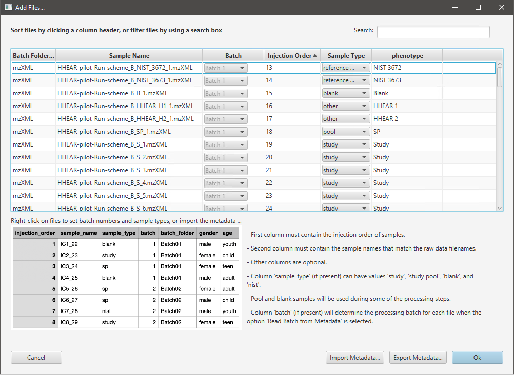
After a workflow and its parameters are chosen, users must select raw data files for the new project by clicking on Select Files... or Select Folder... button. Currently, files in CDF, mzML, mzXML, and ThermoFisher RAW formats are supported. Additionally, the data should be in the centroid mode when mzML or mzXML files are used. Only the ThermoFisher RAW files will be centroided automatically. After users select raw data files, they will see the Add Files window (Figure 2.4) where they can view all samples, adjust the corresponding batches and sample type information, and import and export metadata. ADAP-BIG can import metadata from a CSV file with the columns:
injection_order contains the sample injection information (usually numbers 1, 2, 3,…),
sample_order contains filenames of the raw data files,
sample_type contains the sample type values such as “study”, “sample” for regular samples, “pool”, “study pool”, “sp” for study pool samples, “blank” for blank samples, and “standard”, “nist”, “reference material” for samples with a reference material,
batch (optional) contains the batch number if more than one batch is to be processed (numbers 1, 2, 3,…),
batch_folder (optional) contains names of the folders with the raw data files of each batch (used for checking that each file is assigned to the correct batch)
(optional) other columns with the information on disease-control, gender, weight, etc. (used in PCA and statistical tests)
At the bottom of the Add Files window, users can see an example of the metadata file. Each CSV file must contain columns injection_order and sample_order (in that order), while other columns are optional. After importing a metadata file, users should see all the metadata assigned to the samples in the Add Files window. Moreover, users can export the metadata (e.g., after modifying the batch and sample type information) by clicking the Export Metadata… button. Finally, after clicking the OK button, the New Project window will display per-batch statistics (Figure 2.3) with numbers showing the number of samples with a particular metadata value in each batch. Users are advised to check these numbers to make sure that the metadata is correct.
Finally, users can choose whether the workflow steps should be executed immediately after creating the project (Figure 2.3). If the Execute Entire Workflow checkbox is selected, then all workflow steps will be executed immediately after creating the new project. Otherwise, ADAP-BIG will only import the raw data files without processing them. The latter is useful when users want to only view raw data files or adjust parameters of the workflow steps before running them. After the project is created and the option Execute Entire Workflow was selected, the processing will start immediately and users will see the queued workflow steps in the progress area at the bottom of the main window (Figure 1.2).
Processing Raw MS Data
After an ADAP-BIG project is created, the data processing will start automatically if the option “Execute entire workflow” was selected during the project creation. Users can view the progress of the data processing in the task area at the bottom of the application window (Figure 1.2). Users may still use ADAP-BIG while the processing is running, for example, they can select the Input step to view the raw data while the other workflow steps are being processed. See chapters 4—6 about the available visualization for each workflow step. However, users cannot view the workflow step results until the processing of that step is finished. If users try to view the results of a workflow step that is currently being processed, they will see a message saying that the processing results are not available yet and asking to wait or rerun that workflow step.
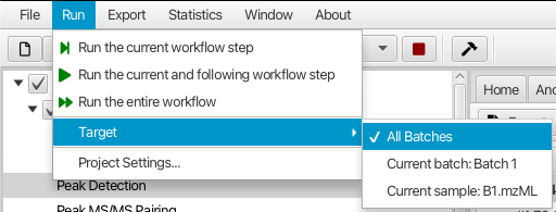
If users need to rerun some of the workflow steps, e.g. after changing their parameters, they can do so by selecting the workflow step in the project tree or the workflow bar, and selecting one of the Run menu options (Figure 2.5). Three options are available to execute workflow steps:
Run the current workflow step will execute only the selected workflow step. This option is useful when users want to try new parameters of a workflow step and see the new processing results without rerunning other workflow steps. However, they need to remember to manually rerun the following steps in order to update the results of those steps.
Run the current and following workflow steps will rerun the workflow steps starting from the selected step. This option is useful when users want to apply new parameters to a workflow step and automatically update the results of that step and all the following steps.
Run the entire workflow will automatically rerun all workflow steps on all samples in the project. This option is useful to make sure that all workflow steps are rerun after changing parameters. However, be advised that it may take a long time to rerun the entire workflow, especially for large projects.
In addition to the three processing options, users can select the processing target: the current sample, the current batch, or all batches (Figure 2.5). Depending on the target selection, the current workflow step will be executed on a single sample, all samples in a single batch, or all samples in all batches, correspondingly. This allows users to quickly try new parameters on a single sample and immediately see the new processing results. However, users need to remember to rerun the current and following steps on all samples after adjusting parameters of any workflow step. The alignment steps, multi-batch steps, and other steps after them will use all samples (in a batch if appropriate) regardless of what target is selected by a user.
Processing Parameters and Metadata
ADAP-BIG has two built-in sets of processing parameters that users can select from when creating a new project: “Default parameters for High-mass resolution data” and “Default parameters for Low-mass-resolution data.” The high-mass-resolution parameters are designed for data from high-resolution mass spectrometers, such as Orbitrap, while the low-mass-resolution parameters are designed for data from low-resolution mass spectrometers, such as quadrupole. Users can also import custom parameters from an XML file by clicking the Import... button in the Settings window. For more information about the XML file with parameters, see Section 7.3.
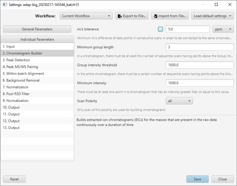
Users can edit parameters for each workflow step either by clicking the Settings button in the visualization tab of any workflow step, selecting menu Run/Settings..., or clicking the settings icon in the toolbar. In all cases, the Settings window will pop up (see Figure 2.6). Here, users can edit the general parameters (that can be applied to multiple workflow steps) or individual parameters of each workflow step.
General Parameters.
ADAP-BIG contains a small number of general parameters that can be applied to multiple workflow steps. The parameter m/z tolerance can be set in ppm or Da, and can be used in the Chromatogram Builder, MS/MS Pairing, and LC-MS Alignment steps. The parameter QC sample type can be set to “blank”, “pool”, or “standard”, and can be used in the Join Aligner, Multi-batch Join Aligner, Background Removal, Normalization, and RSD Filter steps. More general parameters will be added in the future. Users need to remember that using these general parameters is optional, and they can always set the parameters of each workflow step individually. The m/z tolerance and QC sample type parameters for individual steps will have a checkbox to indicate whether the workflow step should use the value of the corresponding general parameter (e.g., see the m/z tolerance parameter of the Chromatogram Builder step in Figure 2.6).
Individual Parameters.
To adjust parameters of an individual workflow step, users can select that workflow step in the list of all processing steps, and change its parameters in the panel on the right of the Settings window. In that panel, each parameter will have a name, value, and a short description. After adjusting parameters, users should click the Save button and rerun the affected workflow steps. Remember, that users must rerun workflow steps for their new parameters to take effect.
Buttons at the top-right of the Settings window let users select the default high-mass-resolution and low-mass-resolution parameters (button Load default settings), import workflow parameters from an existing XML file (button Import from File...), and export the current workflow parameters to an XML file (button Export to File...). This allows users to save and reuse their own custom parameters when needed. Additionally, users have an option to view and edit parameters for the steps of the current workflow (default), GC-MS workflow, LC-MS/MS workflow, multi-batch LC-MS/MS workflow, or view parameters of all workflow steps.
Finally, users may choose to discard their changes by clicking the Reset button or close the Setting window without save by clicking the Close button.
Manage samples in the project.
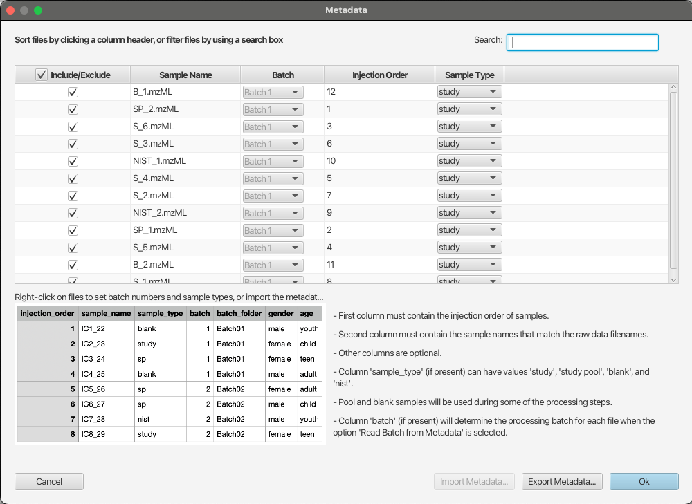
In some situations, users may want to view the sample metadata, exclude certain samples from the processing, or adjust their sample types. In this case, they can click the button Edit Metadata… at the bottom of the project tree to open the Metadata window (Figure 2.7).
In this window, the first column “Include/Exclude” shows what samples are included in the project, and users can uncheck the samples that should not be processed. This doesn’t remove those samples from the project (so users can include them into the project later), but these samples will be ignored during the processing. Users also can update the sample type for each sample by modifying the “Sample Type” column. In order to change multiple samples, it is possible to select multiple rows in the table, and then right-click on any selected row to show the context menu with options to include/exclude samples and change sample types. Finally, users can use the Search box at the top-right of the Metadata window to filter the samples shown in the Metadata window. This filter is convenient to use for finding certain samples based on their filenames (e.g. searching ‘B_‘ to find all blank samples or ‘SP_‘ to find all study pool samples), or their metadata (e.g., searching “control” to find all samples from the control group). In order to search the metadata, make sure that metadata was correctly imported during the creation of the project.
Similar to adjusting parameters, users need to click the “OK” button in the Metadata window and rerun the data processing for the changes to take effect. When excluding samples from the project, users would need to rerun the alignment step and all the steps after the alignment. When changing the sample types of the blank samples, study pool samples, or other quality-control samples, users may need to rerun the Background Removal step and all the steps after it.
Viewing/Exporting Results
After the processing of the entire workflow is complete, users can view and export the processing results and also perform the Principal Component Analysis (PCA). In order to view the final results, users just need to select the last workflow step either in the workflow bar or in the project tree. If the last step is the ANOVA Significance Test but no metadata was imported when creating the project, then the ANOVA Significance Test will not have any results to show. In the latter case, just select the workflow step prior to the significance step.
When processing results are displayed in the main area of ADAP-BIG, users have multiple options to export the results. They can select those options from the main menu Export or at the top-left of the tab with the processing results. Those options include:
Export the quantitation table into a CSV file
Export the MS1 spectra into an MSP file (GC-MS workflow)
Export the MS/MS spectra into an MSP file (single-batch and multi-batch LC-MS/MS workflows)
Export a PDF report with the description of the processing steps and their parameters, and statistics of the processed samples.
Users can use these exported files to perform a statistical analysis or run the library matching. Moreover, then can send the MSP files directly to https://adap.cloud for the library matching by using the option Send to ADAP-KDB in the export menu. In ADAP-KDB, users can identify/annotate the export spectra by matching them against public libraries or private in-house libraries. See https://adap.cloud/about/ for more information about ADAP-KDB.
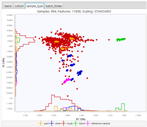
In addition to exporting results, users can also perform some statistical analysis within ADAP-BIG. For example, the ANOVA Statistical Test is a part of the built-in GC-MS and LC-MS/MS workflows. Moreover, user can plot PCA after the last or any other workflow step (as long as that step handles aligned features from multiple samples) by selecting the menu Statistics/Execute PCA (Figure 2.8). In the PCA window, users can choose between intensity and area values, z-scaling and Pareto scaling, coloring by batch, sample type or other available metadata, and also show/hide samples based on their sample types.
Running ADAP-BIG in Terminal and on Cluster
The ADAP-BIG Console App is a standalone Java application that can be run from the command line. The Console App has the same functionality as the GUI version of ADAP-BIG, but it doesn’t have a graphical user interface. Instead, users need to provide a configuration file with the parameters of the workflow steps and the paths to the raw data files. The Console App will process the data according to the parameters in the configuration file and save the results to the specified output directory. Then, users can view the processing results by opening the created project folder in the GUI version of ADAP-BIG.
ADAP-BIG can be run without GUI in a terminal and on a cluster. Running ADAP-BIG on a cluster is useful when users want to process one large dataset or automatically process multiple datasets. To run ADAP-BIG in a terminal, users need to download the ADAP-BIG Console App from the ADAP-BIG website and install Java SE Development Kit 19 or newer if it’s not already installed in your system.
To run ADAP-BIG on a cluster, users need to have access to a cluster with a job scheduler (e.g. SLURM, PBS, SGE), a shared file system (e.g. NFS, Lustre), and Java 19 or newer. When specifying parameters of a job to run the ADAP-BIG Console App on a cluster, consider these guidelines to achieve the best performance:
ADAP-BIG is a multi-threaded Java application, so users should specify the number of threads to use for the processing. Typically, users need to request 1 node, 1 task, and multiple threads/cores/CPUs (e.g. 16, 32, 64) depending on the number of available threads on the node. For example, in SLURM, users need to specify the following parameters:
            #SBATCH --nodes=1
                #SBATCH --ntasks=1
                #SBATCH --cpus-per-task=<number_of_threads>
where <number_of_threads> is the number of threads
to use in parallel (e.g., 16, 32, 64).
ADAP-BIG performs multiple read/write operations during its work, so slow storage may significantly affect the performance. Users should use a high-performance storage space if available. Please consult cluster administrators for the details on the available storage options.
To run the ADAP-BIG Console App in a terminal, users need to open a terminal window and navigate to the directory where the Console App JAR file is located. Then, they can run the Console App with the following command:
        java -Xmx64G -jar adap-big-console-app.jar
                -d PATH-TO-PROJECTS
                -f PATH-TO-SAMPLES
                -w WORKFLOW-FILE
                -s SETTINGS-FILE
                [--factors METADATA-FILE]
where adap-big-console-app.jar is the name of the
Console App JAR file. The console app should be provided the following
command-line arguments:
– the path to the directory where the project will be saved;
– path to the directory with the raw data files (.CDF, .mzML, .mzXML, or ThermoFisher .raw files). If the path contains subfolders, each subfolder will be treated as a separate batch.
– the workflow file, which can be exported from the Workflow Editor in the GUI version of ADAP-BIG (see Section 3.4);
– the settings file, which can be exported from the Settings window in the GUI version of ADAP-BIG (see Section 2.4).
– the metadata file (see Section 2.2 for the description of the metadata file);
When running the ADAP-BIG Console App, users are advised to always
provide the maximum amount of memory available on their system with the
-Xmx option (see the examples). The application will use
the amount of memory specified with the -Xmx option even if
more physical memory is available on the local system, or requested by
the job scheduler. Therefore, pay close attention to the value of the
-Xmx option when running the Console App, and check the log
files to see if the processing steps are using the specified amount of
memory (some steps will use more RAM than the others).
If users are processing a single-batch data, they need to provide
PATH-TO-SAMPLES argument that points to a folder with raw
data files. For example, if the raw data files and metadata file are
located in the directory D:\Data\single-batch-data, the
workflow and settings files are located in D:\configs, and
the project should be created in the directory D:\Projects,
the command to run the ADAP-BIG Console App would be:
    java -Xmx64G -jar adap-big-console-app.jar
            -d D:\Projects
            -f D:\Data\single-batch-data
            -w D:\configs\single-batch-workflow.xml
            -s D:\configs\settings.xml
            --factors D:\Data\single-batch-data\metadata.csv
If users are processing multi-batch data, they need to provide
PATH-TO-SAMPLES argument that points to a folder containing
subfolders with raw data files for each batch. For example, if the raw
data files for the first batch are located in the folder
batch1 inside the directory
D:\Data\multi-batch-data and the raw data files for the
second batch are located in the folder batch2 inside the
directory D:\Data\multi-batch-data, the command to run the
ADAP-BIG Console App would be:
    java -Xmx64G -jar adap-big-console-app.jar
            -d D:\Projects
            -f D:\Data\multi-batch-data
            -w D:\configs\multi-batch-workflow.xml
            -s D:\configs\settings.xml
            --factors D:\Data\multi-batch-data\metadata.csv
The Console App will process the data according to the parameters in the configuration files and save the results to the specified output directory. After the processing is done, users can view the processing results by opening the created project folder in the GUI version of ADAP-BIG.
Processing Workflows
GC-MS Workflow
The GC-MS workflow in ADAP-BIG is designed to process raw untargeted mass spectrometry data, specifically for gas chromatography-mass spectrometry (GC-MS) analysis. The data processing begins with the creation of a new project, where users can select the GC-MS workflow (“Gas Chromatography – Mass Spectrometry”) and select parameters for low-mass-resolution data (“Default parameters for Low-mass resolution data”). Users then add raw data files in CDF format and import metadata to categorize samples. The project setup includes options to execute the entire workflow immediately or adjust parameters before processing.
The first step in the GC-MS workflow is the Input step (see Section 4.1), which imports raw data files and displays their details, including scan information and chromatograms. This step does not have user-defined parameters and serves as the foundation for subsequent processing steps. The Chromatogram Builder step (Section 4.2) follows, constructing extracted-ion chromatograms (EICs) by grouping data points with similar m/z values over time. Users can adjust parameters such as m/z tolerance, group size, and intensity thresholds to optimize chromatogram construction.
Next, the Peak Detection step (Section 4.3) identifies individual peaks within the EICs using parameters like signal-to-noise ratio, peak duration, and wavelet transform coefficients. This step is crucial for detecting distinct peaks that represent analytes in the sample. The Spectral Deconvolution step (Section 4.5) then decomposes these peaks into pure fragmentation mass spectra by clustering similar peaks and constructing model peaks. Users can adjust parameters such as window width, retention time tolerance, and cluster size to refine the deconvolution process.
The GC-MS Alignment step (Section 4.6) aligns similar features across multiple samples based on their retention times and spectral similarities. This step ensures that features are consistently identified across different samples, facilitating comparative analysis. Parameters for this step include sample frequency, retention time tolerance, and matching score thresholds. Finally, the Normalization step (Section 4.9) scales feature intensities and areas to account for variations in sample preparation and instrument response. Users can adjust parameters such as normalization method and pool sample type to standardize feature intensities.
Throughout the workflow, users can view and export processing results, including feature tables and mass spectra. The GC-MS workflow in ADAP-BIG is designed to be flexible and customizable, allowing users to adjust parameters and rerun steps as needed to achieve optimal results. Addition steps like One-way ANOVA test (Section 6.1) and Library Search (Section 6.3) can be added to the default workflow if necessary. The comprehensive visualization and export options facilitate detailed analysis and interpretation of the processed data. See the next chapters for more details about each processing step.
LC-MS/MS Workflow
The LC-MS/MS single-batch workflow in ADAP-BIG is designed to process raw untargeted liquid chromatography-mass spectrometry (LC-MS) data. The data processing begins with the creation of a new project, where users can select the LC-MS workflow “Liquid Chromatography – Tandem Mass Spectrometry (LC-MS(/MS))” and select parameters for high-mass-resolution data (“Default parameters for High-mass resolution data”.) Users then add raw data files in one of the available formats (mzML, mzXML, or raw ThermoFisher data format) and import metadata to categorize samples. The project setup includes options to execute the entire workflow immediately or adjust parameters before processing.
First, the Input step (see Section 4.1) imports raw data files and displays their details, including scan information and chromatograms. This step serves as the foundation for subsequent processing steps and does not have user-defined parameters. Users can view the imported raw data and ensure that all necessary files are correctly loaded before proceeding to the next steps.
The Chromatogram Builder step (Section 4.2) constructs extracted-ion chromatograms (EICs) by grouping data points with similar m/z values over time. Users can adjust parameters such as m/z tolerance, group size, and intensity thresholds to optimize chromatogram construction. This step is crucial for creating a clear representation of the data, allowing for the identification of peaks that represent analytes in the sample. The visualization of this step includes a table of built chromatograms and plots showing the chromatograms and their shapes in the retention time vs. m/z plane.
Following the Chromatogram Builder, the Peak Detection step (Section 4.3) identifies individual peaks within the EICs using parameters like signal-to-noise ratio, peak duration, and wavelet transform coefficients. This step is essential for detecting distinct peaks that represent analytes in the sample. The detected peaks are then paired with the MS/MS scans in the MS/MS Pairing step (Section 4.4), which matches MS/MS scans with the corresponding MS1 peaks. This step is crucial for linking fragmentation spectra to precursor ions and identifying potential compounds.
The LC-MS Alignment step (Section 4.7) aligns similar features across multiple samples based on their retention times and m/z similarities, ensuring consistent identification of features across different samples. Parameters for this step include retention time tolerance, m/z weight, and retention time weight. This step is crucial for comparative analysis, allowing users to see how features vary across samples. The visualization includes tables and plots showing the aligned features and their intensities across samples.
The Background Removal step (Section [section:lcms_background_removal]) removes features based on the ratio of intensities between pool and blank samples. This step is essential for filtering out background noise and ensuring that only relevant features are retained for further analysis. Users can adjust parameters such as pool sample type and blank sample type to customize the background removal process. The visualization includes tables and plots showing the features that passed the background removal.
Finally, The Normalization step (Section 4.9) scales feature intensities and areas to account for variations in sample preparation and instrument response. Users can adjust parameters such as normalization method and pool sample type to standardize feature intensities. This step is crucial for ensuring that features are comparable across samples and that differences in intensity are not due to technical factors.
Throughout the workflow, users can view and export processing results, including feature tables and mass spectra. The LC-MS single-batch workflow in ADAP-BIG is designed to be flexible and customizable, allowing users to adjust parameters and rerun steps as needed to achieve optimal results. Additional steps like Library Matching (Section 6.3) can be added to the default workflow if necessary. The comprehensive visualization and export options facilitate detailed analysis and interpretation of the processed data.
Multi-batch LC-MS/MS Workflow
The multi-batch LC-MS/MS workflow in ADAP-BIG is designed to process raw untargeted liquid chromatography-mass spectrometry (LC-MS) data from multiple batches. The data processing begins with the creation of a new project, where users can select the multi-batch LC-MS/MS workflow “Multi-batch Liquid Chromatography – Tandem Mass Spectrometry (LC-MS(/MS))” and select parameters for high-mass-resolution data (“Default parameters for High-mass resolution data”.) Users then add raw data files in one of the available formats (mzML, mzXML, or raw ThermoFisher data format) and import metadata to categorize samples. The project setup includes options to execute the entire workflow immediately or adjust parameters before processing.
The multi-batch LC-MS/MS workflow builds upon the single-batch LC-MS/MS workflow (Section [section:lcms_workflow]), so its steps from Input through Background Removal are performed for each batch separately. After the Background Removal step, the workflow continues with the Between Batch Alignment step (Section [section:between_batch_alignment]), which aligns features across multiple batches based on their m/z and retention time similarities. This step is crucial for comparing features across different batches and identifying consistent patterns. Parameters for this step include m/z tolerance, retention time tolerance, and alignment score thresholds.
The Multi-batch Normalization step (Section [section:multi_batch_normalization]) scales feature intensities and areas across multiple batches to account for variations in sample preparation and instrument response. Users can adjust parameters such as normalization method and pool sample type to standardize feature intensities. This step is essential for ensuring that features are comparable across batches and that differences in intensity are not due to technical factors.
Following the Normalization, the Batch-effect Correction Step (Section 5.3) removes the batch effect by calculating per-batch shifts for each feature in the log-transformed intensity space. This step is essential for ensuring that differences between batches are not due to technical factors and that features are comparable across batches. Parameters for this step include the missing pool ratio, pool sample type, and whether the results are transformed back to the original space or kept in the log-transformed space.
Finally, the Multi-batch Pool RSD Filter step (Section 5.5) filters out features with a high relative standard deviation (RSD) across pool samples. This step is essential for removing features with high variability and ensuring that only reliable features are retained for further analysis. Parameters for this step include the RSD threshold and the pool sample type. The visualization includes tables and plots showing the features that passed the RSD filter.
Throughout the workflow, users can view and export processing results, including feature tables and mass spectra. The multi-batch LC-MS/MS workflow in ADAP-BIG is designed to be flexible and customizable, allowing users to adjust parameters and rerun steps as needed to achieve optimal results. Additional steps like Library Matching (Section 6.3) can be added to the default workflow if necessary. The comprehensive visualization and export options facilitate detailed analysis and interpretation of the processed data.
Customizing Workflows
Users can customize the GC-MS, LC-MS/MS, and multi-batch LC-MS/MS workflows in ADAP-BIG by adding and removing steps based on their specific data processing needs. The default workflows include a set of processing steps that are commonly used for untargeted mass spectrometry data analysis, but users may want to modify the workflows to include additional steps or exclude unnecessary steps. They can do this by creating or opening an existing project, and then selecting the menu Run/Workflow Editor..., which will open the Workflow Editor window (Fig. 3.1). In this window, users can view all available processing steps and add them to or remove them from the current workflow by clicking the arrow buttons in the center or by dragging and dropping the steps between the left and right panels. By default, all changes will be applied only to the workflow of the current project. If users want to apply these changes to other projects, they can export the updated workflow into an XML file, and then select that file when creating a new project. This allows users to save their custom workflows and reuse them in new projects.
After editing the workflow steps, users can click the Save button to apply the modified workflow to the current project. Additionally, users can export the modified workflow to an XML file by clicking the Export to file... button. This XML file can be selected when creating a new project, instead of the default GC-MS, LC-MS/MS, and multi-batch LC-MS/MS workflows. In the projects that were already created, users can import a custom workflow from an XML file by clicking the Import from file... button in the Workflow Editor window. This allows users to load previously saved custom workflows and apply them to existing projects. The custom workflows can be shared with other users or used across multiple projects to streamline data processing and analysis.
While editing, the workflow can become unfeasible by adding a step that requires the output of a previous step that was removed. For example, the GC-MS Alignment step requires the output of the Spectral Deconvolution step, or Multi-batch Alignment requires the LC-MS Alignment to be performed first for each batch individually. Therefore, removing the Spectral Deconvolution step while keeping the GC-MS Alignment step will turn the current workflow unfeasible. In this case, the Workflow Editor will highlight the problematic steps (the GC-MS Alignment step in this example), show a warning message, and will refuse to save the current workflow. Users will need to fix the workflow by adding the necessary steps back or removing the problematic steps before saving the workflow. Alternatively, users can click the Reset button to discard all changes and revert to the previous workflow or click the Close button to close the Workflow Editor without saving the changes.
Single-batch Processing Steps
Input

Visualization of the Input step is shown on Figure 4.1. The table in the top-left corner displays all scans in a data file including the following information:
automatically generated scan name,
scan number,
can be either MS1 or MS2 (for MS/MS scans),
polarity of scans,
precursor m/z of MS/MS scans,
minimum and maximum m/z values in the scan,
scan retention time (in minutes),
maximum intensity in the scan,
sample name and sample type,
sample metadata if provided.
Users can click on a scan in this table to see its details (bottom-left corner) and its raw spectrum plot (top-right corner). In the bottom-right corner, there are three tabs with the base-ion chromatogram, total-ion chromatogram, and "Retention time vs. m/z" plots. In the base-ion chromatogram plot, intensity at each retention time is equal to the maximum intensity of the scan at that retention time. In the total-ion chromatogram plot, intensity at each retention time is equal to the total intensity of the scan at that retention time. Finally, in the "Retention time vs. m/z" plot, each dot represents pair (ret time, m/z), and its color ranges from white to blue, based on its intensity. In all three plots, the m/z and retention time ranges can changes by using the filter button. Finally, additional samples can be added to the plots by clicking the “+” button. Additionally, double-clicking anywhere in these plots will automatically highlight the scan with the corresponding retention time in the table.
The Input step doesn’t have any user-defined parameters. So, clicking on the Input Settings button will results in opening the Settings window with no workflow step selected. Also, unlike other workflow steps, the Input step doesn’t have any export options.
Chromatogram Builder
This step builds extracted-ion chromatograms (EICs) for the masses that are present in the raw data continuously over a certain duration of time. Users can adjust parameters of the Chromatogram Builder either by clicking button Chromatogram Builder Settings or by selecting menu Run/Settings....
Minimum m/z difference of data points in consecutive scans in order to be connected to the same chromatogram. Twice the m/z tolerance set by the user is the maximum width of a mass trace.
In the entire chromatogram, there must be at least this number of sequential scans having points above the Group intensity threshold set by the user. The optimal value depends on the chromatography system setup. The best way to set this parameter is by studying the raw data and determining what is the typical time span of chromatographic peaks.
See above.
There must be at least one point in the chromatogram that has an intensity greater than or equal to this value.
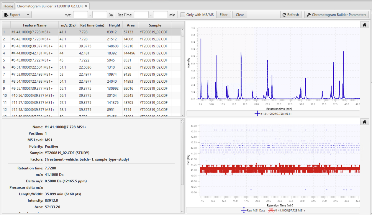
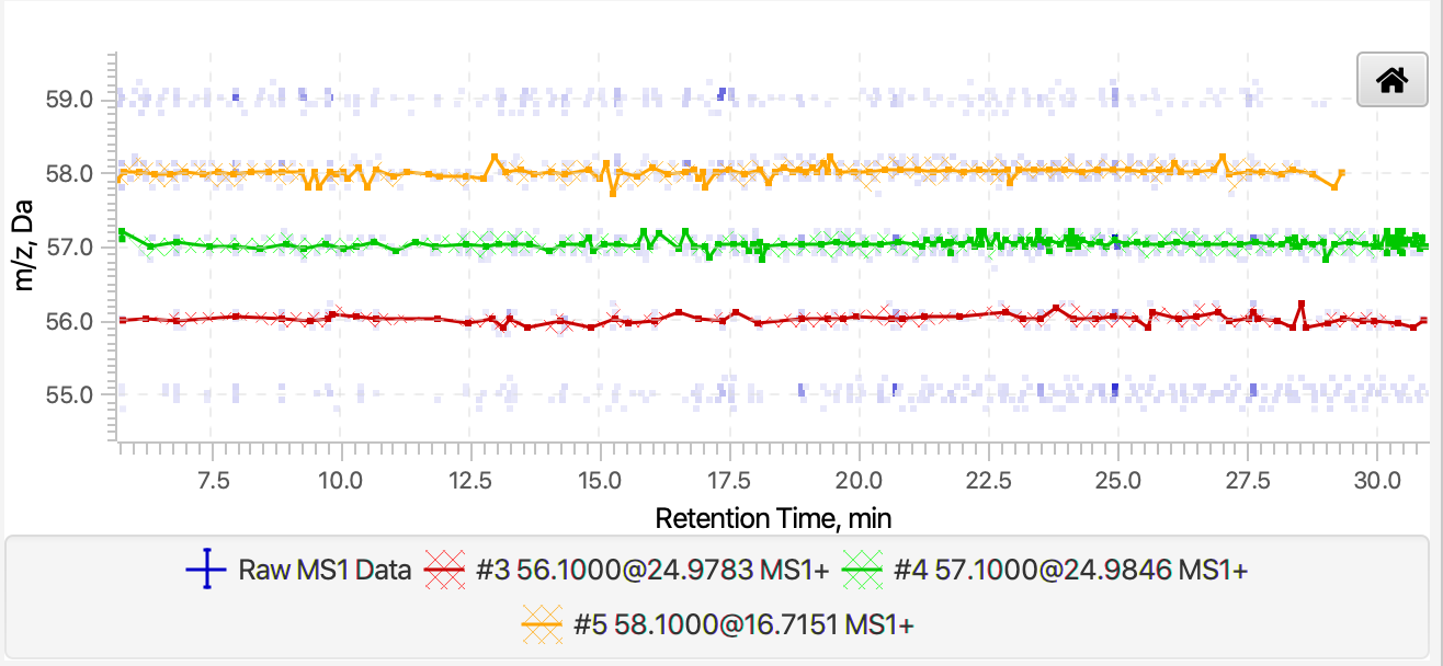
The visualization of the Chromatogram Builder step consists of four parts. The table in the top-left corner shows all built chromatograms with their IDs, names, m/z values, retention times (i.e. the retention time of the highest point in a chromatogram), heights, areas, and sample names. A more detailed information is displayed in the bottom-left corner for the currently selected chromatogram.
The figure at the top-right corner, shows the currently selected chromatogram(s), and the figure at the bottom-right corner, shows the shape of the selected chromatogram(s) in the Retention time vs. m/z plane. The latter figure also displays the near-by raw data points whose color depends on their intensities. This figure can be useful to evaluate the quality of chromatogram. For instance, users can select sort the chromatogram table by the m/z values and select two or more close chromatogram to see how those chromatograms are built (see Figure 4.3). If there is a significant number of data points in between chromatograms, then some chromatograms were missed and users may want to lower the intensity and group size thresholds to build more chromatograms. If there are several chromatograms built over the same cluster of data points, then users may want to increase the m/z tolerance to build fewer chromatograms.
To make it easier for users to find chromatograms, there is a filter at the top of the tab, where users can input an m/z range. After providing m/z range, only chromatograms within that m/z range will be shown in the table. In addition to the m/z range, filter also has fields to input a retention time range and display only the features in MS/MS. This two options will be used in other visualizations (GC-MS and LC-MS/MS), but they are not applicable in the case of the Chromatogram Builder step. So, user can just ignore them for now.
Peak Detection
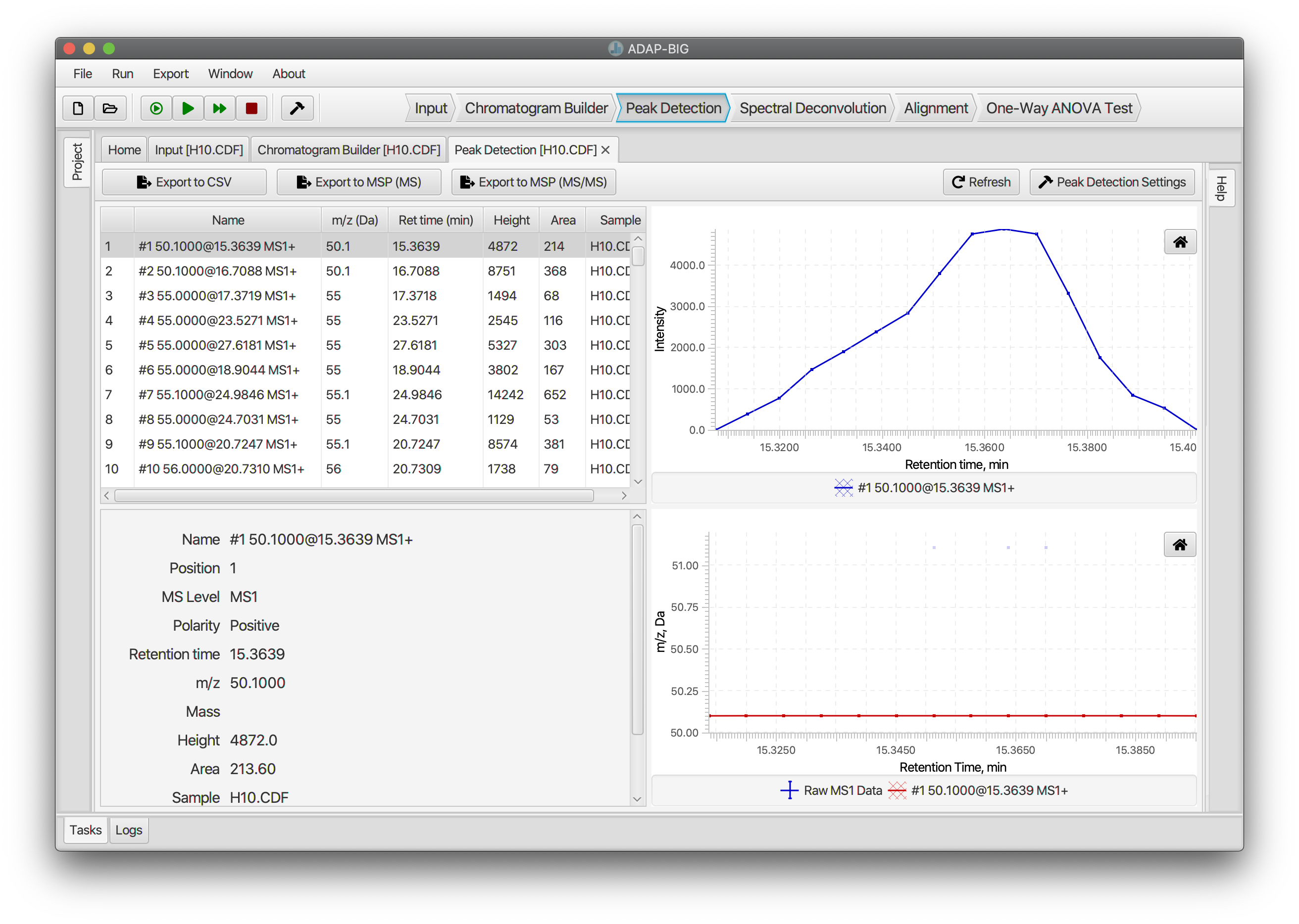
Each EIC that has been constructed spans the entire duration of the chromatography. Peak Detection step detects individual peaks in those EICs. Users can adjust parameters of the Peak Detection either by clicking button Peak Detection Settings or by selecting menu Run/Settings....
the minimum signal-to-noise ratio a peak must have to be considered real. Values grater then or equal to 7 will work well and will only detect a very small number of false positive peaks.
users can choose of two estimators of the signal-to-noise ratio:
intensity_window uses the peak height as the signal level
and the standard deviation of intensities around the peak as the noise
level; wavelet_coefficient uses the continuous wavelet
transform coefficients to estimate the signal and noise level. Analogous
approach is implemented in R-package wmtsa.
the smallest intensity a peak can have and be considered real.
minimum and maximum widths (in minutes) of a peak to be considered real.
this coefficient is found by taking the inner product of the wavelet at the best scale and the peak, and then dividing by the area under the peak. Values around 100 work well for most data.
minimum and maximum widths (in minutes) of the wavelets used for
detecting peaks. The Peak Detection algorithm is highly
sensitive to the upper limit of the RT wavelet range. Also, the
wavelet_coefficient S/N estimator is sensitive to the lower
limit of the RT wavelet range.
The visualization of the Peak Detection step is similar to the visualization of the Chromatogram builder step. See the previous section for details.
MS/MS Pairing (LC-MS)
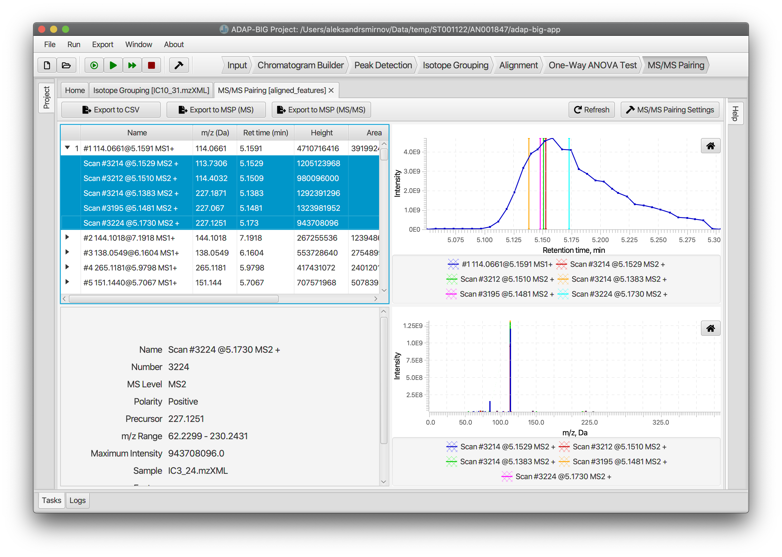
The MS/MS Pairing step finds the MS/MS spectra and pairs them with the aligned components. For MS/MS spectra to be paired with a component, they should satisfy two conditions: (i) the precursor m/z value of an MS/MS spectrum should be contained in the pseudo-spectrum of the component; (ii) the retention time of an MS/MS spectrum should be within the half-height retention time range (i.e. the range corresponding to the upper half of the elution profile) of the component. Users can adjust parameters of the MS/MS Pairing step either by clicking button MS/MS Pairing Settings or by selecting menu Run/Settings....
is used when matching the precursor m/z value of an MS/MS spectrum to m/z values of the pseudo-spectrum of a component.
is used to filter out low-intensity MS/MS spectra. First all MS/MS spectra that satisfy the precursor and retention time requirements are assigned to a component. Then the standard deviation of their intensities is calculated. Finally, if the intensity of an MS/MS spectrum does not exceeds that standard deviated multiplied by the Intensity factor threshold, then that MS/MS spectrum is removed from the component. Users can use value 0 to keep all MS/MS spectra.
The visualization of the MS/MS Pairing step consists of four parts (Figure 4.5). In the top-left corner, there located a table of components. Users can expand each component to see the paired MS/MS spectra. The bottom-left corner contains a panel with detailed information about the selected component or MS/MS spectrum. The fields displayed on that panel change in accordance to whether the selected element is a component or an MS/MS spectrum.
The top-right corner contains a figure that displays an elution profiles of a component (blue curve) and its paired MS/MS spectra (vertical lines). Users must select all MS/MS spectra in the component table to display them on this figure. Finally, the figure in the bottom-right corner displays the pseudo-spectrum of the selected component.
Spectral Deconvolution (GC-MS)
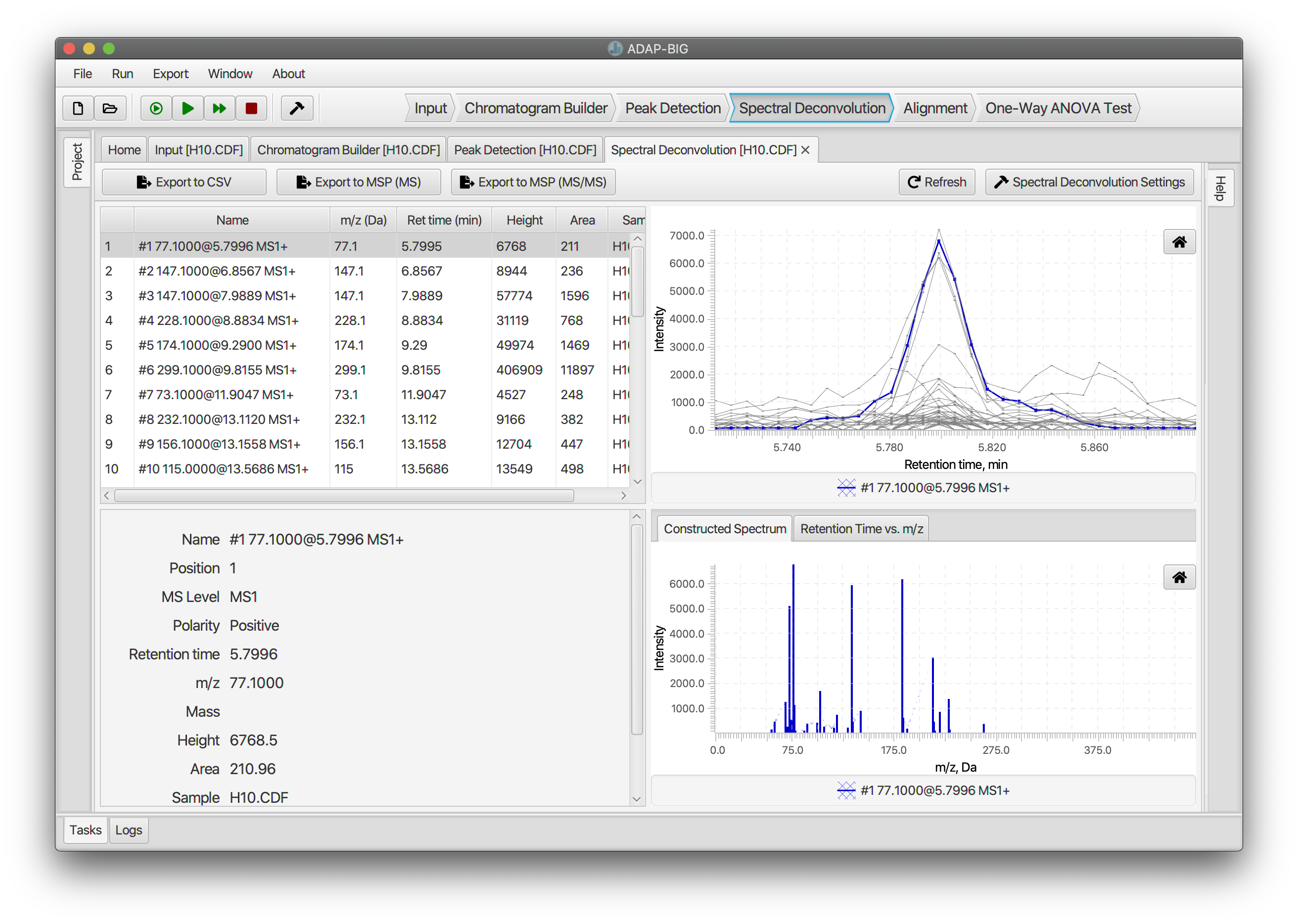
Spectral Deconvolution finds the analytes that are present in a sample and constructs their pure fragmentation mass spectra. Location of analytes is performed in two steps. First, all peaks are assigned to deconvolution windows based on their retention times. Then, in each window, clusters of similar peaks are determined using the similarities of the peak shapes. Then, a model peak is constructed for each cluster, and all peaks are decomposed into a linear combination of the constructed model peaks. Users can adjust parameters of the Spectral Deconvolution either by clicking button Spectral Deconvolution Settings or by selecting menu Run/Settings....
is the maximum length (in minutes) of clusters after the first clustering step. This window width can be chosen based on the width of detected peaks. Typically, value 0.2 works well in most cases.
is the smallest time-gap between any two analytes. The value of this parameter should be a fraction of the average peak width. In our tests, we use 0.04 minutes.
the smallest number of peaks in a single analyte. This parameter depends on a dataset and the number of peaks detected by the previous workflow steps. Typically, its value would range from 1 (if only a few peaks are detected) to 10 or more (if the number of detected peaks is large).
For a unit-mass-resolution data, where coeluting analytes may be present, and a peak typically consists of a hundred or more points, this parameter should be off. For high-mass-resolution data, where coeluting compounds are rare and a peak consists of a few points, this parameter can be turned on.
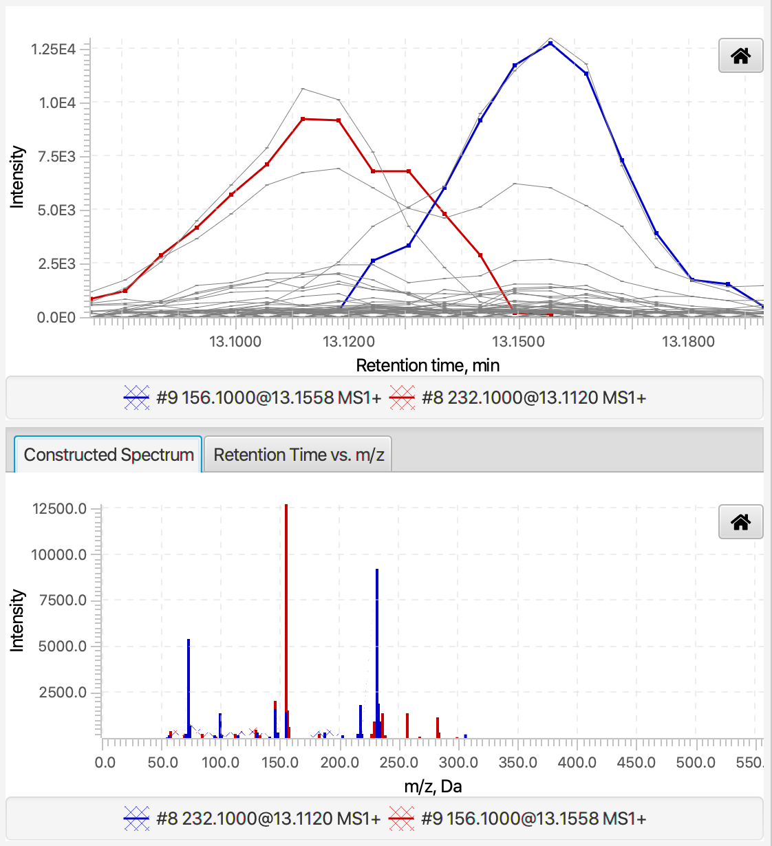
The visualization of the Spectral Deconvolution step consists of four parts. In the upper-left and bottom-left corners are located the table of components and a panel with detailed information about the selected component, respectively. The figures on the right plot the elution profiles and pure fragmentation mass spectra of one or more components (colored curves) and the constituent peaks (grey). This figures help evaluate how peaks are decomposed into linear combinations of the model peaks. To do the later, users can sort the table of components by the retention time and select two or more near-by components. The figures will show the elution profiles of coeluting components and their constructed pure fragmentation spectra (Figure 4.7).
Alignment (GC-MS)
The Alignment step uses uses similarity between constructed mass spectra to find similar components across multiple samples. For this reason, the alignment is performed after the spectral deconvolution step. Users can adjust parameters of the Alignment either by clicking button Alignment Settings or by selecting menu Run/Settings....
takes values between 0 and 1 and equals to the minimum fraction of samples containing aligned components. I.e. if similar components are observed in the fraction of samples less than the minimum sample frequency, then those components are not aligned. If the sample factors are provided than minimum sample frequency is the minimum fraction of samples on one factor group.
is the maximum time-gap between similar components from different samples.
takes values between 0 and 1. Similarity score between components in different samples is determined as follows: \[Score = w\cdot S_{time} + (1-w)\cdot S_{spec},\] where \(S_{time}\) is the relative retention time difference between two components and \(S_{spec}\) the spectral similarity between two components. The score threshold defines the minimum similarity score between two components to be aligned.
takes values between 0 and 1. This parameter is the coefficient \(w\) in the similarity score. If \(w=0\), then only the spectral similarity is used for calculating the similarity of two components. If \(w=1\), then only the retention time difference is used for calculating the similarity of two components. If \(w\) is between 0 and 1, then a weighted combination of the spectral similarity and the retention time difference is used.
is used for matching masses in two mass spectra. This parameter may affect the spectral similarity score.
The top-left corner of the visualization of the Alignment step contains a table of aligned components. In addition to regular table features, users can expand each component to see aligned components from different samples. The figure in the top-right corner displays the elution profiles of aligned components. Users can select all aligned components from different samples to look at their elution profiles together. The figure in the bottom-right corner displays the retention time of the aligned components in the Retention time vs. Sample plane. This figure also displays the maximum difference between retention times of the aligned components. Finally, the bottom-right figure displays intensities of aligned component from each sample.
Alignment (LC-MS)
The Alignment step uses the retention time and m/z similarity to find similar features across multiple samples. This step is performed either right after the peak detection or after the MS/MS pairing step. Users can adjust parameters of the Alignment either by clicking button Alignment Settings or by selecting menu Run/Settings....
specifies the maximum retention time difference (in minutes) allowed between aligned peaks.
determines the contribution of m/z (mass-to-charge ratio) similarity to the alignment score.
determines the contribution of retention time similarity to the alignment score.
specifies the maximum m/z difference (in ppm) allowed between aligned peaks.
if true, the algorithm will keep the non-aligned peaks in the results.
if true, the first pool sample is used as the reference for alignment; otherwise, the largest sample file is used.
specifies the type of sample used as pool samples (e.g., "Pool", "NIST", "QC", "Other").
if true, isotopes are removed at the end of the alignment.
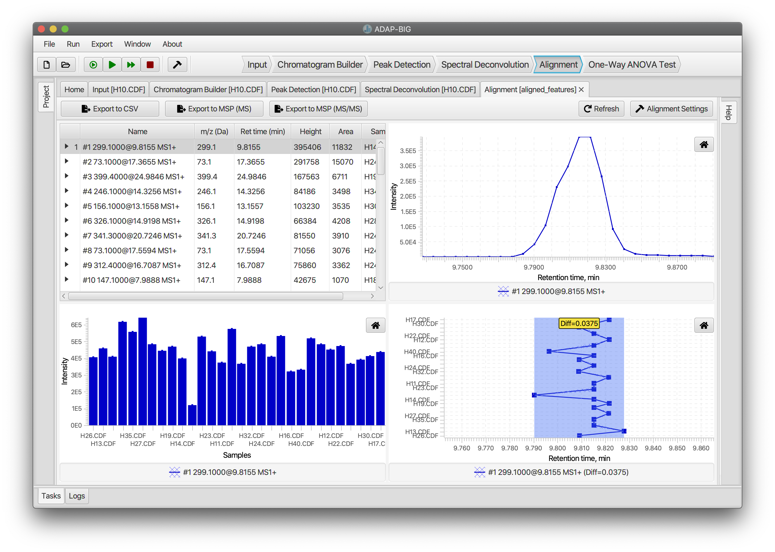
The top-left corner of the visualization of the Alignment step contains a table of aligned features. Clicking one or several features in this table will will update the plots on the right. The top-right corner contains three tabs: "Sample intensities", "Chromatogram", and "MS/MS". The "Sample intensities" tab displays the intensities of the selected features in each sample colored by the sample type, the "Chromatogram" tab displays the elution profile of the selected feature, and the "MS/MS" tab displays the MS/MS spectra paired with the selected feature (if any). The bottom-right corner contains the "Injection-vs-Retention Time" plot, where each dot represents an aligned feature from a sample, and the shaded area represents the stand and end of the retention time range of the selected feature in that sample. This plot can be used to evaluate the retention time differences between aligned features.
Background Removal
The Background Removal step removes the background noise by comparing intensities of each feature in the pool samples to the intensities of that feature in the blank samples. Users can adjust parameters of the Background Removal either by clicking button Background Removal Settings or by selecting menu Run/Settings....
is the minimum ratio of the intensity of a feature in the pool samples to the intensity of that feature in the blank samples. If the ratio is less than the Pool/Blank threshold, then the feature is considered as a background noise and is removed.
is the number of pool samples a feature must be present in to be considered as a signal. If the feature is present in less than the Pool ratio pool samples, then the feature is considered as a background noise and is removed.
is the type of samples used as pool samples (e.g., "Pool", "NIST", "QC", "Other").
The visualization of this step is the same as the visualization of the Alignment step (LC-MS) (Fig. 4.9). See the previous section for details.
Normalization
The Normalization step scales the intensities and areas of the features using one of the two methods:
Total Area Normalization calculates the total area of all features in each sample. Then, it scales the intensities and areas of the features in a sample by dividing them by the total area of that sample and multiplying by the average total area in the pool samples.
Robust Mean Normalization calculates the robust mean of each sample by taking logarithm of the areas of all features in that sample, removing the outliers identified by the Median Absolute Deviation (MAD) method, calculating the mean of the remaining values, and taking the exponent of that mean. Then, it scales the intensities and areas of the features in a sample by dividing them by the robust mean of that sample and multiplying by the average robust mean in the pool samples.
Users can adjust parameters of the Normalization either by clicking button Normalization Settings or by selecting menu Run/Settings....
is the method used for scaling the intensities and areas of the features: “total-intensity” or “log-ratio”.
is the type of samples used as pool samples (e.g., "Pool", "NIST", "QC", "Other"). This parameter can be set individually for this step, or it can use the pool sample type set in the General Parameters (see Section 2.4).
The top-left corner of the visualization of the Normalization step contains a table of normalized features (Fig. 4.10). Clicking one or several features in this table will will update the plots on the right. The top-right corner displays the intensities of the selected features in each sample colored by the sample type. The bottom-right corner shows the normalization factor of the selected feature for each sample. The normalization factors are colored by batch, sample type, or other available metadata.
Pool RSD Filter
The Pool RSD Filter step removes features with a high relative standard deviation (RSD) in the pool samples. Users can adjust parameters of the Pool RSD Filter either by clicking button Pool RSD Filter Settings or by selecting menu Run/Settings....
is the maximum relative standard deviation allowed for a feature to be kept. If the relative standard deviation of a feature in the pool samples is greater than the Relative Standard Deviation Tolerance, then that feature is removed.
is the type of samples used as pool samples (e.g., "Pool", "NIST", "QC", "Other"). This parameter can be set individually for this step, or it can use the pool sample type set in the General Parameters (see Section 2.4).
The visualization of this step is the same as the visualization of the Alignment step (LC-MS) (Fig. 4.9). See the Alignment Step (LC-MS) section for details.
Multi-batch Processing Steps
Between-batch Alignment
Before this step, the features in each batch must be aligned first with the single-batch alignment step (see Section 4.7). If desired, other steps (e.g., the Background Removal) can be applied to each individual batch. After single-batch processing is done, the Between-batch Alignment (LC-MS) step aligns features across multiple batches based on their m/z and retention time similarities.
The parameters of the Between-batch Alignment step are similar to the parameters of the Aliignment Step (LC-MS) and can be adjusted by clicking button Batch Alignment Settings or by selecting menu Run/Settings....
is the maximum retention time difference (in minutes) allowed between aligned features.
determines the contribution of m/z (mass-to-charge ratio) similarity to the alignment score.
determines the contribution of retention time similarity to the alignment score.
specifies the maximum m/z difference allowed between aligned features. This parameter can be specified in ppm or in Da. This parameter can be set individually for this step, or it can use the m/z tolerance set in the General Parameters (see Section 2.4).
if true, the algorithm will keep the unaligned peaks from each batch in the results. Usually, this parameter must be set to true. Otherwise, the algorithm will ignore all features that are not detected in the initial (first) batch.
if true, isotopes are detected in each batch, and only monoisotopic peaks are aligned.
is the minimum fraction of pool samples (across all batches) a feature must be present in to be considered as a signal. If the feature is present in less than the Minimum fraction of pool samples pool samples, then the feature is considered as a background noise and is removed.
is the type of samples used as pool samples (e.g., "Pool", "NIST", "QC", "Other"). This parameter can be set individually for this step, or it can use the pool sample type set in the General Parameters (see Section 2.4).
The visualization of the Between-batch Alignment step is similar to the visualization of the Alignment step (LC-MS) (Fig. 4.9). See the Alignment Step (LC-MS) section for details.
Multi-Batch Normalization
This step is performed in the same way as the single-batch Normalization step (see Section 4.9) with two changes: First, the missing values in each batch are imputed with 10% of the average minimum area across the pool samples in that batch. Second, the average total area/robust mean is calculated across all pool samples from all batches. See section 4.9 for details.
Batch-effect Correction
The Batch-effect Correction step removes the batch effects from the data by following the Broadhurst et al. (2018) method. First, the missting values in each batch are imputed with 10% of the average minimum area across the pool sample in the batch (if it wasn’t already done by the Multi-Batch Normalization step). Then, the log-transform is applied to all area values from all samples. Next, the batch-effect is removed by appying the following steps to each feature: (1) the average area across all pool samples in each batch and the grand average of the areas across all pool samples are calculated; (2) the shift is calculated for each batch by subtracting the grand average area from the batch-specific average area; and (3) the area values are adjusted for each sample by subtracting the shift value from the corresponding batch. Optionally, the data is transformed back to the original scale by taking the exponent of the corrected areas.
The parameters of the Batch-effect Correction step can be adjusted by clicking button Batch-effect Correction Settings or by selecting menu Run/Settings....
is the minimum fraction of pool samples a feature must be present in to be corrected by the batche-effect correction algorithm. If the feature is present in less than the Missing Pool Ratio pool samples, then the feature areas are not corrected.
is the type of samples used as pool samples (e.g., "Pool", "NIST", "QC", "Other"). This parameter can be set individually for this step, or it can use the pool sample type set in the General Parameters (see Section 2.4).
if true, the data is kept in the log-transformed scale after the batch-effect correction. If false, the data is transformed back to the original scale.
The visualization of the Batch-effect Correction step is the same as the visualization of the Between-Batch Alignment step (Fig. 5.1). See the Between-Batch Alignment Step section for details.
ANOVA Batch-effect Correction
The ANOVA Batch-effect Correction step is alternative to the previous Batch-effect Correction Step. It removes the batch effects from the data by removing the features with a significant batch effect. The batch effect is estimated by performing a one-way ANOVA test on the areas of each feature from the pool samples grouped by batch. The features with p-values less than a thershold are removed from.
The parameters of the ANOVA Batch-effect Correction step can be adjusted by clicking button ANOVA Batch-effect Correction Settings or by selecting menu Run/Settings....
is the maximum p-value allowed for a feature to be kept. If the p-value of a feature is less than the PValue cutoff, then that feature is removed.
is the type of samples used as pool samples (e.g., "Pool", "NIST", "QC", "Other"). This parameter can be set individually for this step, or it can use the pool sample type set in the General Parameters (see Section 2.4).
The visualization of the ANOVA Batch-effect Correction step is the same as the visualization of the Between-Batch Alignment step (Fig. 5.1). See the Between-Batch Alignment Step section for details.
Multi-batch Pool RSD Filter
The Multi-batch Pool RSD Filter step is similar to the Pool RSD Filter step (see Section 4.10), but it removes features with a high relative standard deviation (RSD) in the pool samples across all batches. See the Pool RSD Filter section for details.
Post-processing Steps
One-way ANOVA Test
The One-way ANOVA test step performs a one-way ANOVA test on the areas of each feature from the pool samples grouped by a factor imported from the metadata. The p-values of the ANOVA test are calculated for each feature and each factor. The features with p-values less than a threshold are considered as significant.
This step doesn’t have any parameters to adjust.
Dimenstionality Reduction
The Dimenstionality Reduction step applies the Principal Component Analysis (PCA), Partial-Least-Squares Discriminant Analysis (PLS-DA), and Orthogonal Partial-Least-Squares Discriminant Analysis (OPLS-DA) methods, and display results of each method. The PCA method is used for unsupervised analysis, while the PLS-DA and OPLS-DA methods are used for supervised analysis and require selecting the factor of interest, imported from the metadata when the project is created.
Library Search
The Library Search step performs the library search for detected feature through the ADAP-KDB web API. Users have to create an account on the ADAP-KDB website in order to use this feature. Once the account is created, enter your login and password information by going to the menu File/Preferences.... You login information will be stored on your local computer in the encrypted form.
The parameters of the Library Search step can be adjusted by clicking button Library Search Settings or by selecting menu Run/Settings....
if true, the library search will be performed with determining the ontology levels by matching the precursor m/z, retention time, and MS/MS spectra similarity (LC-MS only). If false, the library search will be performed based on the spectral similarity only (GC-MS) or precursor m/z and MS/MS similarity (LC-MS).
is the minimum spectral similarity score on the scale 0—1000 required for a compound to be considered as a match.
is the maximum retention index difference allowed between the detected feature and the library compound.
is the preset of how the retention index should be used in the library search. Users can select one of the following options: “Ignore retention index”, “Penalize matches without retention index (Strong)”, “Penalize matches without retention index (Average)”, “Penalize matches without retention index (Weak)”, “Always match retention index”.
is the maximum m/z difference allowed between the detected feature and the library compound. This parameter can be specified in ppm or in Da. This parameter can be set individually for this step, or it can use the m/z tolerance set in the General Parameters (see Section 2.4).
is the maximum number of library compounds that can be matched to a single detected feature.
is the list of libraries to search in. Users can select one or more libraries from the list of available libraries.
Advanced Functionality
Running individual steps in the command line
ADAP-BIG workflow steps can be executed not only through the ADAP-BIG GUI and Console applications, but also by running individual workflow steps from the command line. In order to do it, users should have Java 9+ installed on their local machine and download the ADAP-BIG jar files available at the GitHub Release page.
Currently, ADAP-BIG include 11 jar files representing each ADAP-BIG workflow step. Below, these jar files are listed together with their command-line arguments:
input.jarimports raw data files into an ADAP-BIG project.–projectpath to the project folder;–inputpath to a raw data file;–factors(optional) path to a CSV file with factor values.chromatogram-builder.jarfinds raw data points with similar m/z and constructs extracted-ion chromatograms.–projectpath to the project folder;–filenamesample name (name of the corresponding raw data file).peak-detection.jardetects peaks in every extracted-ion chromatogram.–projectpath to the project folder;–filenamesample name (name of the corresponding raw data file).spectral-deconvolution.jarforms components and constructs their pure fragmentation mass spectra.–projectpath to the project folder;–filenamesample name (name of the corresponding raw data file).simple-spectral-deconvolution.jargroups similar peaks into components and constructs their pseudo-spectra.–projectpath to the project folder;–filenamesample name (name of the corresponding raw data file).alignment.jarfinds similar components across samples and aligns them–projectpath to the project folder.significance.jarperforms the one-way ANOVA test for each aligned component with the factor groups specified during the raw data import.–projectpath to the project folder;–typetypes of features this module it applied to, can be one ofchromatogram,peak,component,aligned_component;–factor(optional) name of the factor used to calculate the ANOVA test. If no factor is provided, then ANOVA is performed for all available factors.adduct-search.jardetects adducts by matching peaks of the pseudo-spectrum to a list of known adducts and calculates components’ masses.
–projectpath to the project folder;–typetypes of features this module it applied to, can be one ofchromatogram,peak,component,aligned_component.mass-search.jarmatches the computed masses to the RefMet database.
–projectpath to the project folder;–typetypes of features this module it applied to, can be one ofchromatogram,peak,component,aligned_component.ms2-pairing.jarpairs MS/MS spectra to the constructed components.
–projectpath to the project folder;–typetypes of features this module it applied to, can be one ofchromatogram,peak,component,aligned_component.output.jarexports the processing results into CSV or MSP files.
–projectpath to the project folder;–filename(optional) sample name (name of the corresponding raw data file). If not specified, then data for all samples will be exported;–typetypes of features this module it applied to, can be one ofchromatogram,peak,component,aligned_component;–outputname of the file to export data to, this file should have either .csv or .msp extension;–outputlevel(optional) can be either ms1 (for exporting MS1 spectra) or ms2 (for exporting MS/MS spectra).
It should be noted that every jar file has a mandatory argument
–project, which specifies path to the project folder. That
folder should be already exist and contain file
settings.xml containing parameters of the workflow steps.
Users can create such file manually or export it from the ADAP-BIG
application.
Then, each jar file can be executed as following:
java -jar input.jar –project PATH_TO_PROJECT –input RAW_DATA_FILE
where java is Java 9+ command, input.jar
path to an ADAP-BIG jar file, PATH_TO_PROJECT path to the
project folder, and RAW_DATA_FILE path to a raw data file
to be imported.
Editing the workflow.xml
file
|
|---|
workflow.xml.Figure 7.1 shows an
example of file
workflow.xml used by the ADAP-BIG application to store the
GC-MS and LC-MS workflows of processing raw data. However, users can
build custom processing workflows by creating their own
workflow.xml files.
The workflow description file should follow certain rules. First, it
must contain the root XML element called <workflow>.
Then, children of the <workflow> element must have
names matching the full class names of the Java classes of ADAP-BIG
workflow steps. These classes typically similar to the names of the jar
files of the corresponding workflow steps. See the class names in Figure
7.1 and the jar
files described in
Section 7.1 for examples.
In the workflow description file, users can specify the command-line arguments listed in Section 7.1 for each workflow step. However, there are some important differences between the command-line arguments and their counterparts in the workflow description file:
command-line argument
–projectis not specified in the fileworkflow.txtbecause it is added automatically by the ADAP-BIG application prior to every execution of a data processing workflow.arguments
–input,–factors, and–filenamecorrespond to self-closing XML elements<input/>,<factors/>,<filename/>with no content. Their values are assigned by the ADAP-BIG application to the names of raw data files and factors selected in the New Project window of the ADAP-BIG application.all other XML elements are converted into a command-line arguments. ADAP-BIG application converts XML elements of the workflow description file into command-line arguments as follows: element
<tag value="TAG_VALUE">is converted into command-line argument–tag TAG_VALUE.
Below, we list several examples of command-line execution of workflow
steps and their counterparts in file workflow.txt.
Example 1.
Command-line execution of the import of a raw data file
java -jar significance.jar –project PATH_TO_PROJECT –input PATH_TO_FILE
corresponds to the following lines in the workflow description file:
|
Example 2.
Command-line execution of the alignment step
java -jar alignment.jar –project PATH_TO_PROJECT
corresponds to the following line in the workflow description file:
|
Example 3.
Command-line execution of the one-way ANOVA test on all aligned components
java -jar significance.jar –project PATH_TO_PROJECT –type aligned_component
corresponds to the following lines in the workflow description file:
|
Editing the settings.xml
file
|
|---|
settings.xml.Figure 7.2 shows an
example of file
settings.xml used by the ADAP-BIG application and by
individual jar files to store user-defined parameters of every workflow
step. Currently, users can choose between default and unit-mass preset
parameters. However, they can also create a custom settings file with
their own parameters.
The settings file should follow certain rules. First, it must contain
the root XML element called <settings>. Then,
children of the settings> element must have names
matching the full names of the Java classes of ADAP-BIG workflow steps.
This rule should be followed in the file workflow.xml as
well. Next, the children of each workflow step in settings file is
converted into parameters of that workflow step as follows: XML
element
<name type="TYPE" value="VALUE">
is converted into a parameter with name, type, and value
corresponding to attributes name, type, and
value. The tag name name should match one of
the hard-coded parameters of the workflow step. The attribute
type should be one of int,
double, text, boolean. Finally,
the attribute value will be converted into either integer,
real number, boolean in accordance with the specified type.
Currently, there are two additional XML elements for representing a user-defined parameter, that do not follow the above described rule. First, it is possible to specify a range-of-values parameter by using the pattern
<name type="double.range" start="START" end="END">
Second, users can provide a list of adducts for the adduct-search step by using the following pattern:
<adducts type="adduct.list">
        <adduct name="M+2H+Na" num.molecules="1" adduct.mass="25.0038" charge="3"
                quasi.molecular.ion="false"/>
        <adduct name="M+2N+H" num.molecules="1" adduct.mass="46.9857" charge="3"
                quasi.molecular.ion="false"/>
        ...
    </adducts>
Here, attribute name can take any value but is
preferably a user-friendly name of an adduct. Attributes
num.molecules, adduct.mass, and
charge correspond to variables \(n\), \(m\),
and \(q\) defined in the formula \[mz = \frac{n\cdot M - m}{q},\]
where \(M\) is the mass of the original molecule,
and \(mz\) m/z value of the adduct.
Finally, every workflow step must have a corresponding segment in the
settings file. However, that segment may not have any parameters (see
InputModule and SignificanceModule in Figure
7.2). In the latter
case, the
default parameters of that workflow step will be used.